Soit la fonction numérique f f f x x x f ( x ) = x e x − 1 f(x)=x\text e^x - 1 f ( x ) = x e x − 1 C f C_f C f ( O ; i → , j → ) (O;\overrightarrow{i},\overrightarrow{j}) ( O ; i , j ) 2 cm 2~\text{cm} 2 cm
a) Nous devons donner l'ensemble de définition D f D_f D f f f f
Aucune condition n'est imposée sur x x x D f = R \boxed{D_f=\R} D f = R
b) Nous devons calculer lim x → − ∞ f ( x ) \lim\limits_{x\to-\infty}f(x) x → − ∞ lim f ( x )
lim x → − ∞ x e x = 0 (croissances compar e ˊ es) ⟹ lim x → − ∞ ( x e x − 1 ) = − 1 \lim\limits_{x\to-\infty}x~\text e^x=0\quad\text{(croissances comparées)}\quad\Longrightarrow\quad \lim\limits_{x\to-\infty}(x~\text e^x-1)=-1 x → − ∞ lim x e x = 0 (croissances compar e ˊ es) ⟹ x → − ∞ lim ( x e x − 1 ) = − 1 lim x → − ∞ x , e x = 0 (croissances compar e ˊ es) ⟹ lim x → − ∞ f ( x ) = − 1 \phantom{\lim\limits_{x\to-\infty}x,\text e^x=0\quad\text{(croissances comparées)}}\quad\Longrightarrow\quad \boxed{\lim\limits_{x\to-\infty}f(x)=-1} x → − ∞ l i m x , e x = 0 (croissances compar e ˊ es) ⟹ x → − ∞ lim f ( x ) = − 1
Graphiquement, nous déduisons que la courbe C f C_f C f − ∞ -\infty − ∞ y = − 1 y=-1 y = − 1
Nous devons calculer lim x → + ∞ f ( x ) \lim\limits_{x\to+\infty}f(x) x → + ∞ lim f ( x ) lim x → + ∞ f ( x ) x \lim\limits_{x\to+\infty}\dfrac{f(x)}{x} x → + ∞ lim x f ( x )
{ lim x → + ∞ x = + ∞ lim x → + ∞ e x = + ∞ ⟹ lim x → + ∞ x , e x = + ∞ \left\lbrace\begin{matrix}\lim\limits_{x\to+\infty}x=+\infty\\\lim\limits_{x\to+\infty}\text e^x=+\infty\end{matrix}\right.\quad\Longrightarrow\quad \lim\limits_{x\to+\infty}x,\text e^x=+\infty { x → + ∞ lim x = + ∞ x → + ∞ lim e x = + ∞ ⟹ x → + ∞ lim x , e x = + ∞ { lim x → + ∞ x = + ∞ lim x → + ∞ e x = + ∞ ⟹ lim x → + ∞ ( x , e x − 1 ) = + ∞ \phantom{\left\lbrace\begin{matrix}\lim\limits_{x\to+\infty}x=+\infty\\\lim\limits_{x\to+\infty}\text e^x=+\infty\end{matrix}\right.}\quad\Longrightarrow\quad \lim\limits_{x\to+\infty}(x,\text e^x-1)=+\infty { x → + ∞ l i m x = + ∞ x → + ∞ l i m e x = + ∞ ⟹ x → + ∞ lim ( x , e x − 1 ) = + ∞ { lim x → + ∞ x = + ∞ lim x → + ∞ e x = + ∞ ⟹ lim x → + ∞ f ( x ) = + ∞ \phantom{\left\lbrace\begin{matrix}\lim\limits_{x\to+\infty}x=+\infty\\\lim\limits_{x\to+\infty}\text e^x=+\infty\end{matrix}\right.}\quad\Longrightarrow\quad \boxed{\lim\limits_{x\to+\infty}f(x)=+\infty} { x → + ∞ l i m x = + ∞ x → + ∞ l i m e x = + ∞ ⟹ x → + ∞ lim f ( x ) = + ∞
lim x → + ∞ f ( x ) x = lim x → + ∞ x e x − 1 x \lim\limits_{x\to+\infty}\dfrac{f(x)}{x}=\lim\limits_{x\to+\infty}\dfrac{x\text e^x-1}{x} x → + ∞ lim x f ( x ) = x → + ∞ lim x x e x − 1 lim x → + ∞ f ( x ) x = lim x → + ∞ ( x e x x − 1 x ) \phantom{\lim\limits_{x\to+\infty}\dfrac{f(x)}{x}}=\lim\limits_{x\to+\infty}\left(\dfrac{x\text e^x}{x}-\dfrac{1}{x}\right) x → + ∞ l i m x f ( x ) = x → + ∞ lim ( x x e x − x 1 ) lim x → + ∞ f ( x ) x = lim x → + ∞ ( e x − 1 x ) \phantom{\lim\limits_{x\to+\infty}\dfrac{f(x)}{x}}=\lim\limits_{x\to+\infty}\left(\text e^x-\dfrac{1}{x}\right) x → + ∞ l i m x f ( x ) = x → + ∞ lim ( e x − x 1 )
Or { lim x → + ∞ e x = + ∞ lim x → + ∞ 1 x = 0 ⟹ lim x → + ∞ ( e x − 1 x ) = + ∞ \text{Or }\quad \left\lbrace\begin{matrix} \lim\limits_{x\to+\infty}\text e^x=+\infty\\\lim\limits_{x\to+\infty}\dfrac 1x=0 \end{matrix}\right.\quad\Longrightarrow\quad \lim\limits_{x\to+\infty}\left(\text e^x-\dfrac{1}{x}\right)=+\infty Or ⎩ ⎨ ⎧ x → + ∞ lim e x = + ∞ x → + ∞ lim x 1 = 0 ⟹ x → + ∞ lim ( e x − x 1 ) = + ∞ D’o u ˋ lim x → + ∞ f ( x ) x = + ∞ \text{D'où }\quad \boxed{\lim\limits_{x\to+\infty}\dfrac{f(x)}{x}=+\infty} D’o u ˋ x → + ∞ lim x f ( x ) = + ∞
Graphiquement (interprétation hors programme) , nous déduisons que la courbe C f C_f C f
a) Soit f ′ f' f ′ f f f f ′ ( x ) f'(x) f ′ ( x ) f f f
Pour tout réel x x x
f ′ ( x ) = ( x e x − 1 ) ′ f'(x)=(x\text e^x-1)' f ′ ( x ) = ( x e x − 1 ) ′ f ′ ( x ) = ( x e x ) ′ − 0 \phantom{f'(x)}=(x\text e^x)'-0 f ′ ( x ) = ( x e x ) ′ − 0 f ′ ( x ) = x ′ × e x + x × ( e x ) ′ \phantom{f'(x)}=x'\times \text e^x+x\times (\text e^x)' f ′ ( x ) = x ′ × e x + x × ( e x ) ′ f ′ ( x ) = 1 × e x + x × e x \phantom{f'(x)}=1\times \text e^x+x\times \text e^x f ′ ( x ) = 1 × e x + x × e x
f ′ ( x ) = e x + x , e x \phantom{f'(x)}=\text e^x+x,\text e^x f ′ ( x ) = e x + x , e x f ′ ( x ) = ( 1 + x ) e x \phantom{f'(x)}=(1+x)~\text e^x f ′ ( x ) = ( 1 + x ) e x
⟹ ∀ , x ∈ R , f ′ ( x ) = ( 1 + x ) e x \Longrightarrow\quad\boxed{\forall,x\in\R,\quad f'(x)=(1+x)~\text e^x} ⟹ ∀ , x ∈ R , f ′ ( x ) = ( 1 + x ) e x
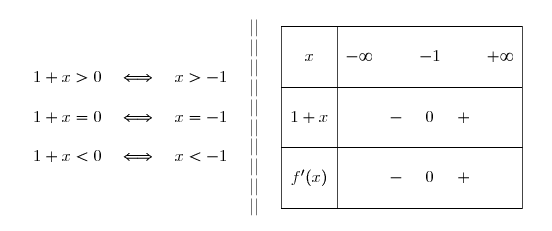
L'exponentielle étant strictement positive sur R \R R f ′ ( x ) f'(x) f ′ ( x ) 1 + x 1+x 1 + x
Nous obtenons ainsi le tableau de signes de f ′ ( x ) f'(x) f ′ ( x )
Par conséquent,
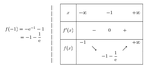
∙ \bullet ∙ x ∈ ] − ∞ ; − 1 [ x\in~]-\infty\;;\;-1[ x ∈ ] − ∞ ; − 1 [ f ′ ( x ) < 0 f'(x)< 0 f ′ ( x ) < 0 ∙ \bullet ∙ x ∈ ] − 1 ; + ∞ [ x\in\,]-1\;;\;+\infty[ x ∈ ] − 1 ; + ∞ [ f ′ ( x ) > 0 f'(x)> 0 f ′ ( x ) > 0 ∙ \bullet ∙ f ′ ( − 1 ) = 0 f'(-1)=0 f ′ ( − 1 ) = 0
b) Nous devons dresser le tableau des variations de f f f
c) Nous devons donner une équation de la tangente ( T ) (T) ( T ) C f C_f C f x = 0 x=0 x = 0
L'équation de cette tangente est de la forme y = f ′ ( 0 ) ( x − 0 ) + f ( 0 ) y=f'(0)(x-0)+f(0) y = f ′ ( 0 ) ( x − 0 ) + f ( 0 ) y = f ′ ( 0 ) x + f ( 0 ) \boxed{y=f'(0)x+f(0)} y = f ′ ( 0 ) x + f ( 0 )
Or { f ( x ) = x , e x − 1 f ′ ( x ) = ( 1 + x ) e x ⟹ { f ( 0 ) = 0 × e 0 − 1 f ′ ( 0 ) = ( 1 + 0 ) e 0 ⟹ { f ( 0 ) = − 1 f ′ ( 0 ) = 1 \left\lbrace\begin{matrix}f(x)=x,\text e^x-1\\f'(x)=(1+x)\,\text e^x\end{matrix}\right.\quad\Longrightarrow\quad\left\lbrace\begin{matrix}f(0)=0\times\text e^0-1\\f'(0)=(1+0)\,\text e^0\end{matrix}\right.\quad\Longrightarrow\quad\left\lbrace\begin{matrix}f(0)=-1\\f'(0)=1\end{matrix}\right. { f ( x ) = x , e x − 1 f ′ ( x ) = ( 1 + x ) e x ⟹ { f ( 0 ) = 0 × e 0 − 1 f ′ ( 0 ) = ( 1 + 0 ) e 0 ⟹ { f ( 0 ) = − 1 f ′ ( 0 ) = 1
D'où une équation de la tangente à ( C f ) (C_f) ( C f ) 0 0 0 y = x − 1 \boxed{y=x-1} y = x − 1
Nous devons construire la tangente ( T ) (T) ( T ) ( C f ) (C_f) ( C f ) ( O ; i → , j → ) (O;\overrightarrow{i},\overrightarrow{j}) ( O ; i , j )
Soit la fonction F F F F ( x ) = x e x − e x − x F(x)=x~\text e^x -\text e^x - x F ( x ) = x e x − e x − x
a) Nous devons justifier que F F F f f f D f D_f D f
La fonction F F F R \R R x ∈ R x\in \R x ∈ R
F ′ ( x ) = ( x , e x − e x − x ) ′ F'(x)=\Big(x,\text e^x -\text e^x - x\Big)' F ′ ( x ) = ( x , e x − e x − x ) ′ F ′ ( x ) = ( x , e x ) ′ − e x − 1 \phantom{F'(x)}=(x,\text e^x)' -\text e^x -1 F ′ ( x ) = ( x , e x ) ′ − e x − 1 F ′ ( x ) = x ′ × e x + x × ( e x ) ′ − e x − 1 \phantom{F'(x)}=x'\times\text e^x+x\times(\text e^x)' -\text e^x -1 F ′ ( x ) = x ′ × e x + x × ( e x ) ′ − e x − 1 F ′ ( x ) = 1 × e x + x × e x − e x − 1 \phantom{F'(x)}=1\times\text e^x+x\times\text e^x -\text e^x -1 F ′ ( x ) = 1 × e x + x × e x − e x − 1
F ′ ( x ) = e x + x , e x − e x − 1 \phantom{F'(x)}=\text e^x+x,\text e^x -\text e^x -1 F ′ ( x ) = e x + x , e x − e x − 1 F ′ ( x ) = x e x − 1 \phantom{F'(x)}=x~\text e^x -1 F ′ ( x ) = x e x − 1 F ′ ( x ) = f ( x ) \phantom{F'(x)}=f(x) F ′ ( x ) = f ( x )
⟹ ∀ x ∈ R F ′ ( x ) = f ( x ) \Longrightarrow\quad\boxed{\forall~x\in\R~\quad F'(x)=f(x)} ⟹ ∀ x ∈ R F ′ ( x ) = f ( x )
Par conséquent, F F F f f f D f = R D_f=\R D f = R
b) Nous devons calculer en cm² l'aire du domaine plan délimité par la courbe ( C f ) (C_f) ( C f ) x = 1 x=1 x = 1 x = ln 4 x=\ln 4 x = ln 4
La fonction f f f [ 1 ; ln 4 ] [1\;;\;\ln 4] [ 1 ; ln 4 ] f ( 1 ) = e − 1 > 0 f(1)=\text e-1 >0 f ( 1 ) = e − 1 > 0
Nous en déduisons que la fonction f f f [ 1 ; ln 4 ] [1\;;\;\ln 4] [ 1 ; ln 4 ]
Donc l'aire demandée se calcule en unité d'aire par ∫ 1 ln 4 f ( x ) d x \displaystyle\int_1^{\ln4}f(x)\,\text dx ∫ 1 l n 4 f ( x ) d x
∫ 1 ln 4 f ( x ) d x = [ F ( x ) ] 1 ln 4 \displaystyle\int_1^{\ln4}f(x)\,\text dx=\Big[F(x)\Big]_1^{\ln4} ∫ 1 l n 4 f ( x ) d x = [ F ( x ) ] 1 l n 4 ∫ 1 ln 4 f ( x ) d x = [ x e x − e x − x ] 1 ln 4 \phantom{\displaystyle\int_1^{\ln4}f(x)\,\text dx}=\Big[x\,\text e^x -\text e^x - x\Big]_1^{\ln4} ∫ 1 l n 4 f ( x ) d x = [ x e x − e x − x ] 1 l n 4 ∫ 1 ln 4 f ( x ) d x = ( ln 4 e ln 4 − e ln 4 − ln 4 ) − ( 1 e 1 − e 1 − 1 ) \phantom{\displaystyle\int_1^{\ln4}f(x)\,\text dx}=\Big({\ln4}\,\text e^{\ln4} -\text e^{\ln4} - {\ln4}\Big) - \Big( 1\,\text e^1 -\text e^1 - 1\Big) ∫ 1 l n 4 f ( x ) d x = ( ln 4 e l n 4 − e l n 4 − ln 4 ) − ( 1 e 1 − e 1 − 1 ) ∫ 1 ln 4 f ( x ) , d x = ( 4 ln 4 − 4 − ln 4 ) − ( e − e − 1 ) \phantom{\displaystyle\int_1^{\ln4}f(x),\text dx}=\Big(4\ln4 -4 - {\ln4}\Big) - \Big( \text e -\text e - 1\Big) ∫ 1 l n 4 f ( x ) , d x = ( 4 ln 4 − 4 − ln 4 ) − ( e − e − 1 )
∫ 1 ln 4 f ( x ) , d x = ( 3 ln 4 − 4 ) − ( − 1 ) \phantom{\displaystyle\int_1^{\ln4}f(x),\text dx}=(3\ln4 -4) - ( - 1) ∫ 1 l n 4 f ( x ) , d x = ( 3 ln 4 − 4 ) − ( − 1 ) ∫ 1 ln 4 f ( x ) , d x = 3 ln 4 − 4 + 1 \phantom{\displaystyle\int_1^{\ln4}f(x),\text dx}=3\ln4 -4+1 ∫ 1 l n 4 f ( x ) , d x = 3 ln 4 − 4 + 1 ∫ 1 ln 4 f ( x ) , d x = 3 ln 4 − 3 \phantom{\displaystyle\int_1^{\ln4}f(x),\text dx}=3\ln4 -3 ∫ 1 l n 4 f ( x ) , d x = 3 ln 4 − 3
⟹ ∫ 1 ln 4 f ( x ) d x = 3 ( ln 4 − 1 ) u.a. \Longrightarrow\quad\boxed{\displaystyle\int_1^{\ln4}f(x)\,\text dx=3(\ln4 -1)\text{ u.a.}} ⟹ ∫ 1 l n 4 f ( x ) d x = 3 ( ln 4 − 1 ) u.a.
Or l'unité de longueur est 2 cm 2~\text{cm} 2 cm 4 cm 2 4~\text{cm}^2 4 cm 2
Par conséquent, l'aire demandée est égale à 4 × 3 ( ln 4 − 1 ) cm 2 4\times3(\ln4 -1)\text{ cm}^2 4 × 3 ( ln 4 − 1 ) cm 2 12 ( ln 4 − 1 ) cm 2 \boxed{12(\ln4 -1)\text{ cm}^2} 12 ( ln 4 − 1 ) cm 2