Soient f f f g g g ] 0 ; + ∞ [ ]0\, ; +\infty[ ] 0 ; + ∞ [ f ( x ) = 1 2 ln 2 x + ln x + x f(x)=\dfrac{1}{2}\ln^2x+\ln x+x f ( x ) = 2 1 ln 2 x + ln x + x g ( x ) = − x − 1 − ln x g(x)=-x-1-\ln x g ( x ) = − x − 1 − ln x
Partie A : Nous devons calculer les limites de g aux bornes de son ensemble de définition.
∙ { lim x → 0 + x = 0 lim x → 0 + ln x = − ∞ ⟹ lim x → 0 + ( − x − 1 − ln x ) = + ∞ ⟹ lim x → 0 + g ( x ) = + ∞ \bullet\ \left\lbrace\begin{matrix}\lim\limits_{x\to0^+}x=0\\\lim\limits_{x\to0^+}\ln x=-\infty\end{matrix}\right.\ \Longrightarrow\ \lim\limits_{x\to0^+}(-x-1-\ln x)=+\infty\ \Longrightarrow\ \boxed{\lim\limits_{x\to0^+}g(x)=+\infty} ∙ { x → 0 + lim x = 0 x → 0 + lim ln x = − ∞ ⟹ x → 0 + lim ( − x − 1 − ln x ) = + ∞ ⟹ x → 0 + lim g ( x ) = + ∞
∙ { lim x → + ∞ x = + ∞ lim x → + ∞ ln x = + ∞ ⟹ lim x → + ∞ ( − x − 1 − ln x ) = − ∞ ⟹ lim x → + ∞ g ( x ) = − ∞ \bullet\ \left\lbrace\begin{matrix}\lim\limits_{x\to+\infty}x=+\infty\\\lim\limits_{x\to+\infty}\ln x=+\infty\end{matrix}\right.\ \Longrightarrow\ \lim\limits_{x\to+\infty}(-x-1-\ln x)=-\infty\ \Longrightarrow\ \boxed{\lim\limits_{x\to+\infty}g(x)=-\infty} ∙ { x → + ∞ lim x = + ∞ x → + ∞ lim ln x = + ∞ ⟹ x → + ∞ lim ( − x − 1 − ln x ) = − ∞ ⟹ x → + ∞ lim g ( x ) = − ∞
La fonction g g g ] 0 ; + ∞ [ ]0 ; +\infty[ ] 0 ; + ∞ [ ] 0 ; + ∞ [ ]0 ; +\infty[ ] 0 ; + ∞ [
g ′ ( x ) = − x ′ − 1 ′ − ( ln x ) ′ = − 1 − 0 − 1 x = − 1 − 1 x = − x − 1 x ⟹ g ′ ( x ) = − x + 1 x g'(x)=-x'-1'-(\ln x)'=-1-0-\dfrac{1}{x}\ =-1-\dfrac{1}{x}=\dfrac{-x-1}{x}\ \Longrightarrow\boxed{g'(x)=-\dfrac{x+1}{x}} g ′ ( x ) = − x ′ − 1 ′ − ( ln x ) ′ = − 1 − 0 − x 1 = − 1 − x 1 = x − x − 1 ⟹ g ′ ( x ) = − x x + 1
x ∈ ] 0 ; + ∞ [ ⟹ { x > 0 x + 1 > 0 ⟹ x + 1 x > 0 ⟹ − x + 1 x < 0 ⟹ g ′ ( x ) < 0 x\in]0\,;\,+\infty[\ \Longrightarrow\ \left\lbrace\begin{matrix}x>0\\x+1>0\end{matrix}\right.\ \Longrightarrow\ \dfrac{x+1}{x}>0\ \Longrightarrow\ -\dfrac{x+1}{x}<0\ \Longrightarrow\ \boxed{g'(x)<0} x ∈ ] 0 ; + ∞ [ ⟹ { x > 0 x + 1 > 0 ⟹ x x + 1 > 0 ⟹ − x x + 1 < 0 ⟹ g ′ ( x ) < 0
Il s'ensuit que la fonction g est strictement décroissante sur l'intervalle ] 0 ; + ∞ [ . ]0 ; +\infty[. ] 0 ; + ∞ [ .
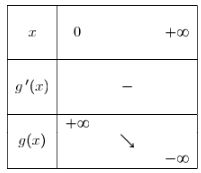
Tableau de variations de g g g
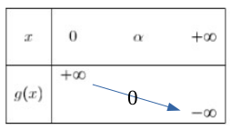
La fonction g est définie, continue et strictement décroissante sur l'intervalle ] 0 , ; , + ∞ [ ]0,;,+\infty[ ] 0 ,;, + ∞ [ lim x → 0 + g ( x ) = + ∞ \lim\limits_{x\to0^+}g(x)=+\infty x → 0 + lim g ( x ) = + ∞ lim x → + ∞ g ( x ) = − ∞ \lim\limits_{x\to+\infty}g(x)=-\infty x → + ∞ lim g ( x ) = − ∞ 0 ∈ g ( ] 0 ; + ∞ [ ) 0\in g(]0\,;\,+\infty[) 0 ∈ g ( ] 0 ; + ∞ [ ) α \alpha α ] 0 , ; , + ∞ [ ]0,;,+\infty[ ] 0 ,;, + ∞ [
Or { g ( 0 , 2 ) = − 0 , 2 − 1 − ln 0 , 2 ≈ 0 , 409 > 0 g ( 0 , 3 ) = − 0 , 3 − 1 − ln 0 , 3 ≈ − 0 , 096 < 0 \text{Or }\left\lbrace\begin{matrix}g(0,2)=-0,2-1-\ln 0,2\approx0,409>0\\g(0,3)=-0,3-1-\ln 0,3\approx-0,096<0\end{matrix}\right. Or { g ( 0 , 2 ) = − 0 , 2 − 1 − ln 0 , 2 ≈ 0 , 409 > 0 g ( 0 , 3 ) = − 0 , 3 − 1 − ln 0 , 3 ≈ − 0 , 096 < 0
D'où 0 , 2 < α < 0 , 3 \boxed{0,2<\alpha<0,3} 0 , 2 < α < 0 , 3
Tableau de variations de g g g
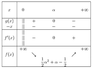
Nous pouvons ainsi déduire le signe de g(x).
∙ \bullet ∙ g ( x ) > 0 g(x) > 0 g ( x ) > 0 − ∞ -\infty − ∞ α \alpha α ∙ \bullet ∙ g ( x ) < 0 g(x) < 0 g ( x ) < 0 ] α ; + ∞ [ ]\alpha ; +\infty[ ] α ; + ∞ [
Partie B : Nous devons calculer les limites de f aux bornes de son ensemble de définition.
∀ , x ∈ , ] 0 , ; , + ∞ [ , , f ( x ) = 1 2 ln 2 x + ln x + x ⟺ ∀ , x ∈ , ] 0 , ; , + ∞ [ , f ( x ) = ln x , ( 1 2 ln x + 1 ) + x \forall,x\in,]0,;,+\infty[,, f(x)=\dfrac{1}{2}\ln^2x+\ln x+x\ \Longleftrightarrow\forall,x\in,]0,;,+\infty[, \boxed{f(x)=\ln x,\left(\dfrac{1}{2}\ln x+1\right)+x} ∀ , x ∈ , ] 0 ,;, + ∞ [ ,, f ( x ) = 2 1 ln 2 x + ln x + x ⟺ ∀ , x ∈ , ] 0 ,;, + ∞ [ , f ( x ) = ln x , ( 2 1 ln x + 1 ) + x
∙ { lim x → 0 + ln x = − ∞ lim x → 0 + ( 1 2 ln x + 1 ) = − ∞ ⟹ lim x → 0 + [ ln x , ( 1 2 ln x + 1 ) + x ] = + ∞ ⟹ lim x → 0 + f ( x ) = + ∞ \bullet\ \left\lbrace\begin{matrix}\lim\limits_{x\to0^+}\ln x=-\infty\\\lim\limits_{x\to0^+}\left(\dfrac{1}{2}\ln x+1\right)=-\infty\end{matrix}\right.\ \Longrightarrow\ \lim\limits_{x\to0^+}\left[\ln x,\left(\dfrac{1}{2}\ln x+1\right)+x\right]=+\infty\ \Longrightarrow\ \boxed{\lim\limits_{x\to0^+}f(x)=+\infty} ∙ ⎩ ⎨ ⎧ x → 0 + lim ln x = − ∞ x → 0 + lim ( 2 1 ln x + 1 ) = − ∞ ⟹ x → 0 + lim [ ln x , ( 2 1 ln x + 1 ) + x ] = + ∞ ⟹ x → 0 + lim f ( x ) = + ∞
∙ { lim x → + ∞ ln x = + ∞ lim x → + ∞ ( 1 2 ln x + 1 ) = + ∞ ⟹ lim x → + ∞ [ ln x , ( 1 2 ln x + 1 ) + x ] = + ∞ ⟹ lim x → + ∞ f ( x ) = + ∞ \bullet\ \left\lbrace\begin{matrix}\lim\limits_{x\to+\infty }\ln x=+\infty\\\lim\limits_{x\to+\infty }\left(\dfrac{1}{2}\ln x+1\right)=+\infty\end{matrix}\right.\ \Longrightarrow\ \lim\limits_{x\to+\infty }\left[\ln x,\left(\dfrac{1}{2}\ln x+1\right)+x\right]=+\infty\ \Longrightarrow\ \boxed{\lim\limits_{x\to+\infty }f(x)=+\infty} ∙ ⎩ ⎨ ⎧ x → + ∞ lim ln x = + ∞ x → + ∞ lim ( 2 1 ln x + 1 ) = + ∞ ⟹ x → + ∞ lim [ ln x , ( 2 1 ln x + 1 ) + x ] = + ∞ ⟹ x → + ∞ lim f ( x ) = + ∞
a) La fonction f est dérivable sur ]0 ; +\infty[ (comme somme de fonctions dérivables sur ]0 ; +\infty[).
f ′ ( x ) = 1 2 ( ln 2 x ) ′ + ( ln x ) ′ + x ′ f'(x)=\dfrac{1}{2}(\ln^2x)'+(\ln x)'+x' f ′ ( x ) = 2 1 ( ln 2 x ) ′ + ( ln x ) ′ + x ′
= 1 2 × 2 ( ln x ) ′ ln x + 1 x + 1 =\dfrac{1}{2}\times2(\ln x)'\,\ln x+\dfrac{1}{x}+1 = 2 1 × 2 ( ln x ) ′ ln x + x 1 + 1
= 1 x ln x + 1 x + 1 =\dfrac{1}{x}\,\ln x+\dfrac{1}{x}+1 = x 1 ln x + x 1 + 1
= ln x + 1 + x x =\dfrac{\ln x+1+x}{x} = x ln x + 1 + x
⟹ ∀ x ∈ ] 0 ; + ∞ [ , f ′ ( x ) = 1 + x + ln x x \Longrightarrow\boxed{\forall\,x\in\,]0\,;\,+\infty[,\,f'(x)=\dfrac{1+x+\ln x}{x}} ⟹ ∀ x ∈ ] 0 ; + ∞ [ , f ′ ( x ) = x 1 + x + ln x
f ′ ( x ) = 1 + x + ln x x = − ( − 1 − x − ln x ) x = − g ( x ) x ⟹ ∀ x ∈ ] 0 ; + ∞ [ , f ′ ( x ) = − g ( x ) x f'(x)=\dfrac{1+x+\ln x}{x}\ =\dfrac{-(-1-x-\ln x)}{x}\ =\dfrac{-g(x)}{x}\\ \Longrightarrow\boxed{\forall\,x\in\,]0\,;\,+\infty[,\,f'(x)=-\dfrac{g(x)}{x}} f ′ ( x ) = x 1 + x + ln x = x − ( − 1 − x − ln x ) = x − g ( x ) ⟹ ∀ x ∈ ] 0 ; + ∞ [ , f ′ ( x ) = − x g ( x )
b) Nous avons montré dans la partie A que α \alpha α
g ( α ) = 0 ⟺ − α − 1 − ln α = 0 ⟺ ln α = − α − 1 g(\alpha)=0\Longleftrightarrow -\alpha-1-\ln \alpha=0\ \Longleftrightarrow \ln \alpha=-\alpha-1 g ( α ) = 0 ⟺ − α − 1 − ln α = 0 ⟺ ln α = − α − 1
D'où { ln α = − α − 1 ln 2 α = ( − α − 1 ) 2 ⟺ { ln α = − α − 1 ln 2 α = α 2 + 2 α + 1 \left\lbrace\begin{matrix} \ln \alpha=-\alpha-1\\ \ln^2 \alpha=(-\alpha-1)^2\end{matrix}\right.\ \Longleftrightarrow\ \left\lbrace\begin{matrix} \ln \alpha=-\alpha-1\\ \ln^2 \alpha=\alpha^2+2\alpha+1\end{matrix}\right. { ln α = − α − 1 ln 2 α = ( − α − 1 ) 2 ⟺ { ln α = − α − 1 ln 2 α = α 2 + 2 α + 1
Par conséquent,
f ( α ) = 1 2 ln 2 α + ln α + α f(\alpha)=\dfrac{1}{2}\ln^2\alpha+\ln \alpha+\alpha f ( α ) = 2 1 ln 2 α + ln α + α
= 1 2 ( α 2 + 2 α + 1 ) + ( − α − 1 ) + α =\dfrac{1}{2}(\alpha^2+2\alpha+1)+(-\alpha-1)+\alpha\ = 2 1 ( α 2 + 2 α + 1 ) + ( − α − 1 ) + α
= 1 2 α 2 + α + 1 2 − α − 1 + α =\dfrac{1}{2}\alpha^2+\alpha+\dfrac{1}{2}-\alpha-1+\alpha = 2 1 α 2 + α + 2 1 − α − 1 + α
= 1 2 α 2 + α − 1 2 ⟹ f ( α ) = 1 2 α 2 + α − 1 2 =\dfrac{1}{2}\alpha^2+\alpha-\dfrac{1}{2}\\ \Longrightarrow\boxed{f(\alpha)=\dfrac{1}{2}\alpha^2+\alpha-\dfrac{1}{2}} = 2 1 α 2 + α − 2 1 ⟹ f ( α ) = 2 1 α 2 + α − 2 1
Nous savons que pour tout x x x ] 0 ; + ∞ [ , ]0 ; +\infty[, ] 0 ; + ∞ [ , f ′ ( x ) = − g ( x ) x = g ( x ) − x f'(x)=-\dfrac{g(x)}{x}=\dfrac{g(x)}{-x} f ′ ( x ) = − x g ( x ) = − x g ( x ) f f f
Nous devons étudier le comportement de ( C f ) (C_f) ( C f )
a) ∙ \bullet ∙ lim x → + ∞ f ( x ) x \lim\limits_{x\to+\infty}\dfrac{f(x)}{x} x → + ∞ lim x f ( x )
lim x → + ∞ f ( x ) x = lim x → + ∞ 1 2 ln 2 x + ln x + x x = lim x → + ∞ ( 1 2 ln 2 x x + ln x x + x x ) ⟹ lim x → + ∞ f ( x ) x = lim x → + ∞ ( 1 2 , ln 2 x x + ln x x + 1 ) \lim\limits_{x\to+\infty}\dfrac{f(x)}{x}=\lim\limits_{x\to+\infty}\dfrac{\frac{1}{2}\ln^2x+\ln x+x}{x}\ =\lim\limits_{x\to+\infty}\left(\dfrac{\frac{1}{2}\ln^2x}{x}+\dfrac{\ln x}{x}+\dfrac{x}{x}\right)\ \Longrightarrow\boxed{\lim\limits_{x\to+\infty}\dfrac{f(x)}{x}=\lim\limits_{x\to+\infty}\left(\dfrac{1}{2},\dfrac{\ln^2x}{x}+\dfrac{\ln x}{x}+1\right)} x → + ∞ lim x f ( x ) = x → + ∞ lim x 2 1 ln 2 x + ln x + x = x → + ∞ lim ( x 2 1 ln 2 x + x ln x + x x ) ⟹ x → + ∞ lim x f ( x ) = x → + ∞ lim ( 2 1 , x ln 2 x + x ln x + 1 )
Calculons lim x → + ∞ ln 2 x x \lim\limits_{x\to+\infty}\dfrac{\ln^2x}{x} x → + ∞ lim x ln 2 x x = t 2 x = t^2 x = t 2
lim x → + ∞ ln 2 x x = lim t → + ∞ ln 2 t 2 t 2 = lim t → + ∞ ln t 2 × ln t 2 t 2 = lim t → + ∞ 2 ln t × 2 ln t t 2 = 4 × lim t → + ∞ ln t t × ln t t = 4 × 0 × 0 ( croissances compar e ˊ es ) = 0 ⟹ lim x → + ∞ ln 2 x x = 0 \lim\limits_{x\to+\infty}\dfrac{\ln^2x}{x}=\lim\limits_{t\to+\infty}\dfrac{\ln^2t^2}{t^2}\ =\lim\limits_{t\to+\infty}\dfrac{\ln t^2\times \ln t^2}{t^2}\ =\lim\limits_{t\to+\infty}\dfrac{2\ln t\times 2\ln t}{t^2}\ =4\times\lim\limits_{t\to+\infty}\dfrac{\ln t}{t}\times\dfrac{\ln t}{t}=4\times0\times0\ (\text{croissances comparées})\ =0\ \Longrightarrow\boxed{\lim\limits_{x\to+\infty}\dfrac{\ln^2x}{x}=0} x → + ∞ lim x ln 2 x = t → + ∞ lim t 2 ln 2 t 2 = t → + ∞ lim t 2 ln t 2 × ln t 2 = t → + ∞ lim t 2 2 ln t × 2 ln t = 4 × t → + ∞ lim t ln t × t ln t = 4 × 0 × 0 ( croissances compar e ˊ es ) = 0 ⟹ x → + ∞ lim x ln 2 x = 0
D'où, en utilisant ce dernier résultat et les croissances comparées, nous obtenons :
lim x → + ∞ f ( x ) x = lim x → + ∞ ( 1 2 , ln 2 x x + ln x x + 1 ) = 1 2 × 0 + 0 + 1 = 1 ⟹ lim x → + ∞ f ( x ) x = 1 \lim\limits_{x\to+\infty}\dfrac{f(x)}{x}=\lim\limits_{x\to+\infty}\left(\dfrac{1}{2},\dfrac{\ln^2x}{x}+\dfrac{\ln x}{x}+1\right)=\dfrac{1}{2}\times0+0+1=1\ \Longrightarrow\boxed{\lim\limits_{x\to+\infty}\dfrac{f(x)}{x}=1} x → + ∞ lim x f ( x ) = x → + ∞ lim ( 2 1 , x ln 2 x + x ln x + 1 ) = 2 1 × 0 + 0 + 1 = 1 ⟹ x → + ∞ lim x f ( x ) = 1
∙ \bullet ∙ lim x → + ∞ ( f ( x ) − x ) \lim\limits_{x\to+\infty}(f(x)-x) x → + ∞ lim ( f ( x ) − x )
lim x → + ∞ ( f ( x ) − x ) = lim x → + ∞ ( 1 2 ln 2 x + ln x + x − x ) = lim x → + ∞ ( 1 2 ln 2 x + ln x ) = lim x → + ∞ ln x , ( 1 2 ln x + 1 ) Or lim x → + ∞ ln x = + ∞ ⟹ lim x → + ∞ ln x , ( 1 2 ln x + 1 ) = + ∞ D’o u ˋ lim x → + ∞ ( f ( x ) − x ) = + ∞ \lim\limits_{x\to+\infty}(f(x)-x)=\lim\limits_{x\to+\infty}\left(\dfrac{1}{2}\ln^2x+\ln x+x-x\right)\ =\lim\limits_{x\to+\infty}\left(\dfrac{1}{2}\ln^2x+\ln x\right)\ =\lim\limits_{x\to+\infty}\ln x,\left(\dfrac{1}{2}\ln x+1\right)\ \text{Or }\lim\limits_{x\to+\infty}\ln x=+\infty\ \Longrightarrow\ \lim\limits_{x\to+\infty}\ln x,\left(\dfrac{1}{2}\ln x+1\right)=+\infty\ \text{D'où }\boxed{\lim\limits_{x\to+\infty}(f(x)-x)=+\infty} x → + ∞ lim ( f ( x ) − x ) = x → + ∞ lim ( 2 1 ln 2 x + ln x + x − x ) = x → + ∞ lim ( 2 1 ln 2 x + ln x ) = x → + ∞ lim ln x , ( 2 1 ln x + 1 ) Or x → + ∞ lim ln x = + ∞ ⟹ x → + ∞ lim ln x , ( 2 1 ln x + 1 ) = + ∞ D’o u ˋ x → + ∞ lim ( f ( x ) − x ) = + ∞
Nous en déduisons que ( C f ) (C_f) ( C f ) y = x y = x y = x + ∞ +\infty + ∞
b) Soit ( D ) (D) ( D ) y = x y = x y = x ( C f ) (C_f) ( C f ) f ( x ) − x f ( x ) − x f ( x ) − x
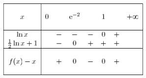
f ( x ) − x = 1 2 ln 2 x + ln x + x − x = 1 2 ln 2 x + ln x = ln x ( 1 2 ln x + 1 ) ⟹ f ( x ) − x = ln x ( 1 2 ln x + 1 ) f(x)-x=\dfrac{1}{2}\ln^2x+\ln x+x-x\ =\dfrac{1}{2}\ln^2x+\ln x\ =\ln x\,\left(\dfrac{1}{2}\ln x+1\right)\ \Longrightarrow\boxed{f(x)-x=\ln x\,\left(\dfrac{1}{2}\ln x+1\right)} f ( x ) − x = 2 1 ln 2 x + ln x + x − x = 2 1 ln 2 x + ln x = ln x ( 2 1 ln x + 1 ) ⟹ f ( x ) − x = ln x ( 2 1 ln x + 1 )
Tableau de signes de f ( x ) − x f ( x ) − x f ( x ) − x
Par conséquent,
∙ \bullet ∙ e − 2 e^{-2} e − 2 ( C f ) (C_f) ( C f ) ∙ \bullet ∙ e − 2 e^{-2} e − 2 ( C f ) (C_f) ( C f ) ∙ \bullet ∙ ( C f ) (C_f) ( C f )
Représentation graphique de ( C f ) (C_f) ( C f )
Soit F F F ] 0 ; + ∞ [ ]0 ; +\infty[ ] 0 ; + ∞ [ F ( x ) = 1 2 x ln 2 x + x 2 2 F(x)=\dfrac{1}{2}\,x\,\ln^2x+\dfrac{x^2}{2} F ( x ) = 2 1 x ln 2 x + 2 x 2
a) Vérifions que F F F f f f ] 0 ; + ∞ [ ]0 ; +\infty[ ] 0 ; + ∞ [ ] 0 ; + ∞ [ ]0 ; +\infty[ ] 0 ; + ∞ [
F ′ ( x ) = 1 2 ( x ln 2 x ) ′ + 1 2 ( x 2 ) ′ F^{\prime}(x)=\dfrac{1}{2}\left(x\,\ln^2 x\right)'+\frac{1}{2}(x^2)' F ′ ( x ) = 2 1 ( x ln 2 x ) ′ + 2 1 ( x 2 ) ′
= 1 2 [ x ′ × ln 2 x + x × ( ln 2 x ) ′ ] + 1 2 × 2 x =\dfrac{1}{2}\,\left[x'\times\ln^2x+x\times(\ln^2x)'\right]+\dfrac{1}{2}\times2x\ = 2 1 [ x ′ × ln 2 x + x × ( ln 2 x ) ′ ] + 2 1 × 2 x
= 1 2 [ 1 × ln 2 x + x × 2 × ( ln x ) ′ × ln x ] + x =\dfrac{1}{2}\,\left[1\times\ln^2x+x\times2\times(\ln x)'\times\ln x\right]+x = 2 1 [ 1 × ln 2 x + x × 2 × ( ln x ) ′ × ln x ] + x
= 1 2 [ ln 2 x + x × 2 × ( 1 x ) × ln x ] + x =\dfrac{1}{2}\,\left[\ln^2x+x\times2\times\left(\dfrac{1}{x}\right)\times\ln x\right]+x = 2 1 [ ln 2 x + x × 2 × ( x 1 ) × ln x ] + x
= 1 2 [ ln 2 x + 2 ln x ] + x =\dfrac{1}{2}\left[\ln^2x+2\,\ln x\right]+x = 2 1 [ ln 2 x + 2 ln x ] + x
= 1 2 ln 2 x + ln x + x =\dfrac{1}{2}\ln^2x+\ln x+x = 2 1 ln 2 x + ln x + x
= f ( x ) ⟹ ∀ x ∈ ] 0 ; + ∞ [ , F ′ ( x ) = f ( x ) =f(x)\ \Longrightarrow\boxed{\forall\ x\in\,]0\,;\,+\infty[,\ F^{\prime}(x)=f(x)} = f ( x ) ⟹ ∀ x ∈ ] 0 ; + ∞ [ , F ′ ( x ) = f ( x )
D'où, la fonction F est une primitive de f f f ] 0 ; + ∞ [ ]0 ; +\infty[ ] 0 ; + ∞ [
b) L'aire A \mathscr{A} A 2 ^2 2 ( C f ) (C_f) ( C f ) x = 1 x = 1 x = 1 x = 3 x = 3 x = 3 A = ∫ 1 3 ( 1 2 ln 2 x + ln x + x ) d x \mathscr{A}=\displaystyle\int_{1}^{3}\left(\dfrac{1}{2}\ln^2x+\ln x+x\right)\,\mathrm dx A = ∫ 1 3 ( 2 1 ln 2 x + ln x + x ) d x
A = ∫ 1 3 ( 1 2 ln 2 x + ln x + x ) d x \mathscr{A}=\displaystyle\int_{1}^{3}\left(\dfrac{1}{2}\ln^2x+\ln x+x\right)\,\mathrm dx A = ∫ 1 3 ( 2 1 ln 2 x + ln x + x ) d x
= ∫ 1 3 1 2 ln 2 x d x + ∫ 1 3 ln x d x + ∫ 1 3 x d x =\displaystyle\int_{1}^{3}\dfrac{1}{2}\ln^2x\,\mathrm dx+\displaystyle\int_{1}^{3}\ln x\,\mathrm dx+\displaystyle\int_{1}^{3}x\,\mathrm dx = ∫ 1 3 2 1 ln 2 x d x + ∫ 1 3 ln x d x + ∫ 1 3 x d x
Calculons ∫ 1 3 1 2 ln 2 x d x \displaystyle\int_{1}^{3}\dfrac{1}{2}\ln^2x\,\mathrm dx ∫ 1 3 2 1 ln 2 x d x
Formule de l’int e ˊ grale par parties ‾ : \underline{\text{Formule de l'intégrale par parties}}\ :\ Formule de l’int e ˊ grale par parties :
∫ 1 3 u ( x ) v ′ ( x ) d x \displaystyle\int_{1}^{3} u(x)v'(x)\,\mathrm dx ∫ 1 3 u ( x ) v ′ ( x ) d x
= [ u ( x ) v ( x ) ] 1 3 − ∫ 1 3 u ′ ( x ) v ( x ) d x . =\left[u(x)v(x)\right]_1^{3}-\displaystyle\int_{1}^{3} u'(x)v(x)\,\mathrm dx. = [ u ( x ) v ( x ) ] 1 3 − ∫ 1 3 u ′ ( x ) v ( x ) d x .
avec { u ( x ) = 1 2 ln 2 x ⟹ u ′ ( x ) = 1 2 × 2 × 1 x × ln x = ln x x v ′ ( x ) = 1 ⟹ v ( x ) = x \\ \left\lbrace\begin{matrix}u(x)=\dfrac{1}{2}\ln^2x\\ \Longrightarrow\ u'(x)=\dfrac{1}{2}\times2\times\dfrac{1}{x}\times\ln x=\dfrac{\ln x}{x}\ v'(x)=1\ \Longrightarrow\ v(x)=x\end{matrix}\right. ⎩ ⎨ ⎧ u ( x ) = 2 1 ln 2 x ⟹ u ′ ( x ) = 2 1 × 2 × x 1 × ln x = x ln x v ′ ( x ) = 1 ⟹ v ( x ) = x
Dès lors,
∫ 1 3 1 2 ln 2 x d x \displaystyle\int_{1}^{3}\dfrac{1}{2}\ln^2x\,\mathrm dx ∫ 1 3 2 1 ln 2 x d x
= [ 1 2 x ln 2 x ] 1 3 − ∫ 1 3 ln x x × x d x = [ 1 2 x ln 2 x ] 1 3 − ∫ 1 3 ln x d x =\left[\dfrac{1}{2}\,x\ln^2x\right]_1^{3}- \displaystyle\int_1^{3} \dfrac{\ln x}{x}\times x\,\mathrm dx\ =\left[\dfrac{1}{2}\,x\ln^2x\right]_1^{3}- \displaystyle\int_1^{3}\ln x\,\mathrm dx = [ 2 1 x ln 2 x ] 1 3 − ∫ 1 3 x ln x × x d x = [ 2 1 x ln 2 x ] 1 3 − ∫ 1 3 ln x d x
= [ 1 2 × 3 ln 2 3 − 1 2 × 1 ln 2 1 ] − ∫ 1 3 ln x d x =\left[\dfrac{1}{2}\times3\ln^23-\dfrac{1}{2}\times1\ln^21\right]- \displaystyle\int_1^{3}\ln x\,\mathrm dx = [ 2 1 × 3 ln 2 3 − 2 1 × 1 ln 2 1 ] − ∫ 1 3 ln x d x
= [ 1 2 × 3 ln 2 3 − 0 ] − ∫ 1 3 ln x d x =\left[\dfrac{1}{2}\times3\ln^23-0\right]- \displaystyle\int_1^{3}\ln x\,\mathrm dx = [ 2 1 × 3 ln 2 3 − 0 ] − ∫ 1 3 ln x d x
= 3 2 ln 2 3 − ∫ 1 3 ln x , d x ⟹ ∫ 1 3 1 2 ln 2 x d x = 3 2 ln 2 3 − ∫ 1 3 ln x , d x =\dfrac{3}{2}\ln^23- \displaystyle\int_1^{3}\ln x,\mathrm dx\\ \Longrightarrow\boxed{\displaystyle\int_{1}^{3}\dfrac{1}{2}\ln^2x\,\mathrm dx=\dfrac{3}{2}\ln^23- \displaystyle\int_1^{3}\ln x,\mathrm dx} = 2 3 ln 2 3 − ∫ 1 3 ln x , d x ⟹ ∫ 1 3 2 1 ln 2 x d x = 2 3 ln 2 3 − ∫ 1 3 ln x , d x
Par conséquent,
A = ∫ 1 3 1 2 ln 2 x d x + ∫ 1 3 ln x d x + ∫ 1 3 x d x \mathscr{A}=\displaystyle\int_{1}^{3}\dfrac{1}{2}\ln^2x\,\mathrm dx+\displaystyle\int_{1}^{3}\ln x\,\mathrm dx+\displaystyle\int_{1}^{3}x\,\mathrm dx A = ∫ 1 3 2 1 ln 2 x d x + ∫ 1 3 ln x d x + ∫ 1 3 x d x
= ( 3 2 ln 2 3 − ∫ 1 3 ln x d x ) + ∫ 1 3 ln x d x + ∫ 1 3 x d x =\left(\dfrac{3}{2}\ln^23- \displaystyle\int_1^{3}\ln x\,\mathrm dx\right)+\displaystyle\int_{1}^{3}\ln x\,\mathrm dx+\displaystyle\int_{1}^{3}x\,\mathrm dx = ( 2 3 ln 2 3 − ∫ 1 3 ln x d x ) + ∫ 1 3 ln x d x + ∫ 1 3 x d x
= 3 2 ln 2 3 − ∫ 1 3 ln x d x + ∫ 1 3 ln x d x + ∫ 1 3 x d x =\dfrac{3}{2}\ln^23- \displaystyle\int_1^{3}\ln x\,\mathrm dx+\displaystyle\int_{1}^{3}\ln x\,\mathrm dx+\displaystyle\int_{1}^{3}x\,\mathrm dx = 2 3 ln 2 3 − ∫ 1 3 ln x d x + ∫ 1 3 ln x d x + ∫ 1 3 x d x
= 3 2 ln 2 3 + ∫ 1 3 x d x =\dfrac{3}{2}\ln^23+\displaystyle\int_{1}^{3}x\,\mathrm dx = 2 3 ln 2 3 + ∫ 1 3 x d x
= 3 2 ln 2 3 + [ x 2 2 ] 1 3 = 3 2 ln 2 3 + ( 3 2 2 − 1 2 2 ) =\dfrac{3}{2}\ln^23+\left[\dfrac{x^2}{2}\right]_1^3=\dfrac{3}{2}\ln^23+\left(\dfrac{3^2}{2}-\dfrac{1^2}{2}\right) = 2 3 ln 2 3 + [ 2 x 2 ] 1 3 = 2 3 ln 2 3 + ( 2 3 2 − 2 1 2 )
= 3 2 ln 2 3 + ( 9 2 − 1 2 ) =\dfrac{3}{2}\ln^23+\left(\dfrac{9}{2}-\dfrac{1}{2}\right) = 2 3 ln 2 3 + ( 2 9 − 2 1 )
= 3 2 ln 2 3 + 4 ⟹ A = ( 3 2 ln 2 3 + 4 ) cm 2 ≈ 5 , 81 cm 2 =\dfrac{3}{2}\ln^23+4\\ \Longrightarrow\boxed{\mathscr{A}=\left(\dfrac{3}{2}\ln^23+4\right)\ \text{cm}^2\approx5,81\ \text{cm}^2} = 2 3 ln 2 3 + 4 ⟹ A = ( 2 3 ln 2 3 + 4 ) cm 2 ≈ 5 , 81 cm 2