Étude complète d’une fonction logarithmique (2)

Partie I

1. La fonction $h$ définie sur $]0;+\infty[$ $\text{ par : }$ $h(x)=x^2-\ln x$ est dérivable sur $]0;+\infty[$ comme somme de fonctions dérivables sur cet intervalle $.$

D'où , pour tout réel $x$ strictement positif $\text{ : }$

$\begin{matrix}h'(x)&=&(x^2-\ln x)'&=&(x^2)'-(\ln x)'&=&2x-\dfrac{1}{x}&=&\dfrac{2x^2-1}{x}\end{matrix}$

$\boxed{ h'(x)=\dfrac{2x^2-1}{x} \text{ pour tout } x \text{ de }]0;+\infty[ }$

2. Puisque $x\in]0;+\infty[$ $\text{ , alors le signe de }$ $h'(x)$ est celui de $2x^2-1$ , de plus , on sait que :

Pour tout $x\in]0;+\infty[$ $\text{ : }$ $2x^2-1=\left(\sqrt{2}x\right)^2-1 =(\sqrt{2}x-1)(\sqrt{2}x+1)$

Et , pour tout $x\in]0;+\infty[$ $\text{ : }$ $\sqrt{2} x+1 >0$

Alors le signe de $h'(x)$ est finalement celui de $\sqrt{2}x-1$ , on trace le tableau de signe :

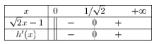
\begin{array}{|c|ccccc|} \hline x & 0 & & 1/\sqrt{2} & & +\infty \ \hline \sqrt{2}x-1 &\dbarre & - & \barre{0} & +& \ \hline h'(x) &\dbarre & - & \barre{0} & +& \ \hline \end{array}

On obtient :

$\boxed{\begin{matrix} \text{ Pour tout }x\in\left] 0;\dfrac{1}{\sqrt{2}}\right]\text{ : }h'(x)\leq 0 \\text{ Pour tout }x\in\left[\dfrac{1}{\sqrt{2}};+\infty\right[\text{ : }h'(x)\geq 0\end{matrix}}$

3. On a directement :

$\begin{matrix}h\left(\dfrac{1}{\sqrt{2}}\right)&=&\left(\dfrac{1}{\sqrt{2}}\right)^2-\ln \left(\dfrac{1}{\sqrt{2}}\right)&=&\dfrac{1}{2} +\ln (\sqrt{2}) \\&=& \dfrac{1}{2}+\ln \left(2^{1/2}\right) &=&\dfrac{1}{2}+\dfrac{1}{2}\ln 2 \\&=&\boxed{ \dfrac{1+\ln 2}{2}}\end{matrix}$

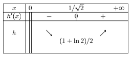
Et on dresse le tableau de variations de $h$ :

$\begin{array}{|c|cccccc|} \hline x & 0 & & & 1/\sqrt{2} & & +\infty \\ \hline h'(x) &\dbarre& &- & \barre{0} & + & \\ \hline & \dbarre& & & & & \ h &\dbarre & & \searrow && \nearrow& \ & \dbarre&& &(1+\ln 2)/2& & \ & \dbarre&& && & \\ \hline \end{array}$

4. On déduit du tableau de variations que le minimum de la fonction $h$ sur $]0;+\infty[$ est $\dfrac{1+\ln 2}{2}$ $.$

On a alors pour tout $x$ de $]0;+\infty[$ $\text{ , }$ $h(x) \geq \dfrac{1+\ln 2}{2}$ $.$ De plus , $\dfrac{1+\ln 2}{2}>0$

D'où :

$\boxed{\forall x\in]0;+\infty[\text{ : }h(x)>0}$

Partie II

La fonction $f$ est définie sur $]0;+\infty[$ $\text{ par : }$ $f(x)=\dfrac{1+\ln x}{x}+x$

1-a) Puisque $\displaystyle\lim_{x\to 0^{+}}\ln x =-\infty$ $\enskip\text{ , donc }$ $\displaystyle\lim_{x\to 0^{+}}\ln x + 1 =-\infty$

De plus , $\displaystyle\lim_{x\to 0^{+}}\dfrac{1}{x} =+\infty$ $\enskip\text{ , d'où }\enskip$ $\displaystyle\lim_{x\to 0^{+}}\dfrac{\ln x+1}{x} =\displaystyle\lim_{x\to 0^{+}}\dfrac{1}{x}\times (\ln x +1) =(+\infty) \times(-\infty )=-\infty$

D'où : $\displaystyle\lim_{x\to 0^{+}}f(x) =\displaystyle\lim_{x\to 0^{+}}\dfrac{1+\ln x}{x}+x=-\infty$

$\boxed{\displaystyle\lim_{x\to 0^{+}}f(x) =-\infty}$

b) Interprétation graphique :

$\boxed{\text{ L'axe des ordonnées est une asymptote verticale à la courbe }(\mathcal{C})\text{ de }f}$

2-a) Puisque $\displaystyle\lim_{x\to +\infty} \dfrac{\ln x}{x} =0$ $\enskip\text{ et }\enskip$ $\displaystyle\lim_{x\to +\infty} \dfrac{1}{x} =0$

Alors :$\displaystyle\lim_{x\to +\infty}f(x) =\displaystyle\lim_{x\to +\infty}\dfrac{1+\ln x}{x}+x=\displaystyle\lim_{x\to +\infty}\dfrac{1}{x}+\dfrac{\ln x}{x}+x=0+0+\infty=+\infty$

$\boxed{\displaystyle\lim_{x\to +\infty}f(x) =+\infty}$

b) On a :

$\displaystyle\lim_{x\to +\infty}f(x)-x =\displaystyle\lim_{x\to +\infty}\dfrac{1+\ln x}{x}+x-x=\displaystyle\lim_{x\to +\infty}\dfrac{1}{x}+\dfrac{\ln x}{x}=0$

$\boxed{\displaystyle\lim_{x\to +\infty}f(x)-x =0}$

c) Interprétation graphique :

$\boxed{\text{ La droite d'équation }y=x \text{ est une asymptote oblique à la courbe }(\mathcal{C})\text{ au voisinage de }+\infty}$

3-a) $f$ est une fonction dérivable sur $]0;+\infty[$ comme quotient et somme de fonctions dérivables sur cet intervalle , alors :

$\begin{matrix}\forall x\in]0;+\infty[\text{ : }f'(x)&=&\left(\dfrac{1+\ln x}{x}+x\right)'&=& \dfrac{(1+\ln x)'x-(1+\ln x)}{x^2}+1\\&=& \dfrac{\dfrac{1}{x}\times x-(1+\ln x)}{x^2}+1&=& \dfrac{1-1-\ln x}{x^2}+1\\&=& \dfrac{-\ln x+x^2}{x^2}&=&\dfrac{x^2-\ln x}{x^2}\end{matrix}$

Donc :
$\boxed{f'(x)=\dfrac{h(x)}{x^2} \text{ , pour tout }x\text{ de }]0;+\infty[ }$

b) On a vu en $4)$ de la partie I que : $\forall x\in]0;+\infty[\text{ : }h(x)>0$

Et puisque $x^2>0$ pour tout $x\in]0;+\infty[$ , alors :

$\forall x\in]0;+\infty[\text{ : }f'(x)>0$

On obtient donc :

$\boxed{\text{ La fonction }f\text{ est strictement croissante sur }]0;+\infty[}$

4-a) On a :

$\begin{matrix} f\left(\dfrac{1}{e}\right) &=&\dfrac{1+\ln \left(\dfrac{1}{e}\right)}{\dfrac{1}{e}}+\dfrac{1}{e}&=&e(1+\ln(e^{-1}))+\dfrac{1}{e}\\&=&e(1-\ln e)+\dfrac{1}{e}&=&e(1-1)+\dfrac{1}{e}\\&=&\dfrac{1}{e}\end{matrix}$

$\boxed{f\left(\dfrac{1}{e}\right)=\dfrac{1}{e}}$

b) Pour tout $x\in]0;+\infty[$ $\enskip\text{ : }\enskip$ $\begin{matrix} f(x)-x&=&\dfrac{1+\ln x}{x}\end{matrix}$

Et puisque $x>0$ $\text{ , alors }$ le signe de $f(x)-x$ est celui de $1+\ln x$ $.$

D'autre part : $1+\ln x\geq 0 \iff \ln x\geq -1 \iff x\geq e^{-1}\iff x\geq \dfrac{1}{e}$

Et $1+\ln x\leq 0 \iff x\leq \dfrac{1}{e}$

On en déduit que :

$\boxed{\begin{matrix} \forall x\in \left]0;\dfrac{1}{e}\right]\text{ : }f(x)-x\leq 0 \ \forall x\in \left[\dfrac{1}{e};+\infty\right[\text{ : }f(x)-x\geq 0 \end{matrix}}$

c) On déduit de ce qui précède , que :

$\boxed{\begin{matrix} (\mathcal{C})\text{ est en dessous de }(\Delta)\text{ sur } \left]0;\dfrac{1}{e}\right] \ (\mathcal{C})\text{ est au-dessus de }(\Delta)\text{ sur } \left[\dfrac{1}{e};+\infty\right[ \ (\mathcal{C})\text{ coupe }(\Delta)\text{ au point }\left(\dfrac{1}{e};\dfrac{1}{e}\right)\end{matrix}}$

5-a) Puisque $x\in\left[\dfrac{1}{e};1\right]$ $\text{ , }$ une primitive de $\dfrac{1}{x}$ est $\ln x$ $.$

On a alors :

$\begin{matrix}\displaystyle\int_{\frac{1}{e}}^{1}\dfrac{1}{x}\text{ d}x &=&\left[\ln x\right]_{\frac{1}{e}}^{1} &=& \ln 1 -\ln \left(\dfrac{1}{e}\right) \\&=& 0-(-\ln e) &=& \ln e \\&=& 1 \end{matrix}$

Et :

$\begin{matrix}\displaystyle\int_{\frac{1}{e}}^{1}\dfrac{\ln x}{x}\text{ d}x &=&\displaystyle\int_{\frac{1}{e}}^{1}\dfrac{1}{x}\times \ln x\text{ d}x&=&\displaystyle\int_{\frac{1}{e}}^{1}\left(\ln x\right)'\ln x \text{ d}x \\&=& \left[\dfrac{\ln ^2 x}{2}\right]_{\frac{1}{e}}^{1} &=& \dfrac{\ln ^2 (1)}{2}-\dfrac{\ln ^2 \left(\dfrac{1}{e}\right)}{2} \\&=& -\dfrac{1}{2}(-\ln e )^2 &=& -\dfrac{1}{2} \end{matrix}$

$\boxed{\displaystyle\int_{\frac{1}{e}}^{1}\dfrac{1}{x}\text{ d}x =1\enskip\enskip\text{ et }\enskip\enskip \displaystyle\int_{\frac{1}{e}}^{1}\dfrac{\ln x}{x}\text{ d}x=-\dfrac{1}{2}}$

b) L'aire de la partie hachurée qui est délimité par la courbe $(\mathcal{C})$ et la droite $(\Delta)$ et les droites d'équations $x=\dfrac{1}{e}$ $\text{ et }$ $x=1$ est en unités d'aire (UA) :

$\displaystyle \int_{1/e}^{1} |f(x)-y|\text{ d}x=\displaystyle \int_{1/e}^{1} |f(x)-x|\text{ d}x$

Et d'après $4$-$b)$ , $f(x)-x\geq 0$ $\text{ , pour tout }$ $x\in\left[\dfrac{1}{e}; 1 \right]$

L'aire de la partie hachurée est en unité d'aire (UA) :

$\begin{matrix}\displaystyle \int_{1/e}^{1} |f(x)-x|\text{ d}x&=&\displaystyle \int_{1/e}^{1} f(x)-x\text{ d}x&=&\displaystyle \int_{1/e}^{1} \dfrac{1+\ln x}{x}\text{ d}x\\&=&\displaystyle \int_{1/e}^{1} \dfrac{1}{x}+\dfrac{\ln x}{x}\text{ d}x &=&\displaystyle \int_{1/e}^{1} \dfrac{1}{x} \text{ d}x +\displaystyle \int_{1/e}^{1} \dfrac{\ln x}{x}\text{ d}x \\&=&1-\dfrac{1}{2} &=&\dfrac{1}{2}\end{matrix}$

$\boxed{\text{ L'aire de la partie hachurée vaut en unité d'aire }\dfrac{1}{2}\enskip(UA)}$